Foundations of AI: Module 3 – Introducing Deep Learning

Table of Contents

Brief Overview

Building upon my earlier posts on Artificial Intelligence where I discussed a subfield of AI called Machine Learning, it is time to examine another exciting part of AI called Deep Learning. But before we proceed, let’s take a moment to recap…

• Artificial Intelligence encompasses the broader concept of creating machines/computers/systems that can perform tasks that usually require human intelligence.
• Machine Learning is a subfield of AI that can learn and make predictions based on patterns observed in a given data set. The classical Machine Learning process requires human intervention to teach the system whether the predicted output is correct.

What is Deep Learning?

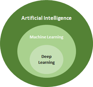
Deep Learning is a subfield of Machine Learning. Therefore, the relationship between Artificial Intelligence, Machine Learning, and Deep Learning can be shown as follows:

What makes Deep Learning captivating is its utilisation of several layers of algorithms within structures known as neural network that mimics the working of the human brain. Through this ‘setup’, the system can autonomously arrive at an accurate decision by automating the feature extraction piece. This is done with phenomenal accuracy, sometimes superseding human capabilities, without human intervention.

For example, imagine we are building a machine that can differentiate between Cabbages and Carrots. In the case of classic machine learning, we must tell the machine the features that distinguish both, such as size, shape, and colour. In deep learning, the system automatically determines these features without human intervention.

What is the typical setup of a Deep Learning based model?

Deep learning-based models primarily rely on architectures related to neural networks. Due to this, neural networks are often referred to as the ‘backbone’ of deep learning. They are called “neural”, as they simulate how neurons in the human brain signal each other. Furthermore, the reference to “deep” in Deep Learning is to indicate that the overall neural ‘setup’ involves more than three layers, including the inputs and output, similar to the image below taken from Bikash Kumar Sundaray LinkedIn article which can be found here:

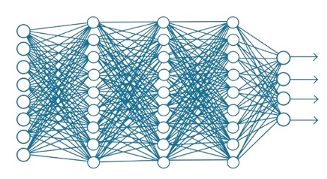
The first set of vertical ‘circles’ (or first tier) is referred to as the “Input Layer” while the last set is the “Output Layer”. In between the two are the “Hidden Layers” which in our case, there are three. In reality, there may be hundreds of hidden layers. 

Every circle, or neuron, has its own knowledge that enables it to generate an output based on the data supplied.  

Raw data is fed to the input layer. Each neuron in the input layer analyses and processes the data supplied based on its knowledge and generates an output, which is then supplied to the first hidden layer.

How does this setup work?

As indicated in the diagram above, the output of each neuron in the input layer is fed as an input to each neuron in the first hidden layer, thus the so many “connecting lines” (channels) in the diagram. 

Each neuron in the first hidden layer analyse and process the data received and generates an output, which is again fed to each neuron in the second hidden layer. This process keeps repeating until it reaches the “output” layer. 

This setup is what is referred to as a traditional feedforward neural network. There are specialised networks, such as the Convolutional Neural Network (CNN), that the direct connections between neurons from one layer to the next do not apply. 

What information is required for the network to learn?

The neural network is fed with a huge amount of input data and the correct output. Rules are also defined to help the network learn. 

For example, imagine we are building a face recognition system that can indicate if the person has a moustache. For the system to learn, the neural network is fed with:

1. Images of people with and without a moustache, and
2. The actual images from this same data set (i.e., the same set of images) of the people with a moustache.

We can stop there, but to make the learning process faster, we might assign a rule instructing the network not to look at the entire image but look underneath the nose and above the mouth. 

How do learning work?

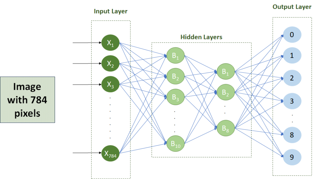
Let’s imagine we are building a number recognition system that can recognise the number on a 784-pixel image. 

Setup

Each pixel will be fed to an input neuron in the input layer, thus, the input layer will have 784 neurons.

The output layer will contain the numbers 0 to 9, therefore, the output layer will be made up of 10 neurons.

In between the input and output layers, hidden layers will be trained to ‘map’ the data fed in the input layer to the correct output neuron.

The setup will look something like this (for simplicity, I assume there are only two hidden layers).

Mechanism

The information will flow from one node to another through channels. Each channel has a value/weight attached to it, while each neuron has a unique number called Bias (referred to as B in the diagrams above and below).

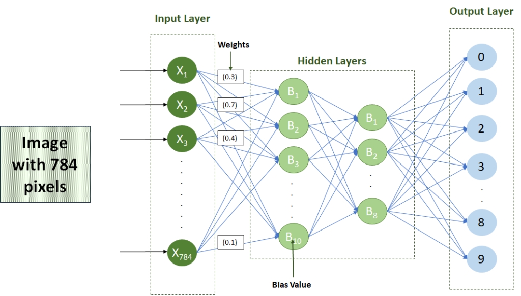
The inputs are then multiplied with the corresponding weight, and their sum is added to the neuron’s bias value.

i.e., for the first neuron in the first hidden layer, the algorithm will be:

(X₁ * 0.3 + X₂ * 0.7 + X₃ * 0.4 + … + X₇₈₄ * 0.1)

The result of this algorithm will be fed to what is called the “Activation Function” which will determine whether the neuron should be “switched on” (i.e., activated). Switched-on neurons will transmit data to the neurons of the next layer as per the connected channels. 

This mechanism will continue to be repeated, and the highest value in the output layer determines the model’s output – i.e., in our example, what in the model’s view is the number on the image. 

Iterative learning

In the initial stages of the learning process, both the bias values and the weights will be incorrect, resulting in the wrong output.

However, remember that we would have provided the model with the correct output. The system’s job is to automatically adjust the bias values and weights so that the model’s output will become equivalent to the correct output. This is done through a series of what are called forward and back propagations.

With all these adjustments happening autonomously, the learning cycle takes time and requires a lot of data for effective training and accurate predictions. However, the benefits are enormous. We have already seen huge advancements in medical research, industrial automation, and aerospace and defence.  Ethical challenges including data privacy and biasing in algorithms remain a challenge, however, despite all this, the journey of deep learning is far from over. 

I have only scratched the surface of deep learning in this post but stay tuned for more information!

As the objective of this post is to offer newcomers in the field of Technology a foundational understanding, I have intentionally simplified certain aspects of the content. If you seek more comprehensive and precise information, please don’t hesitate to reach out.